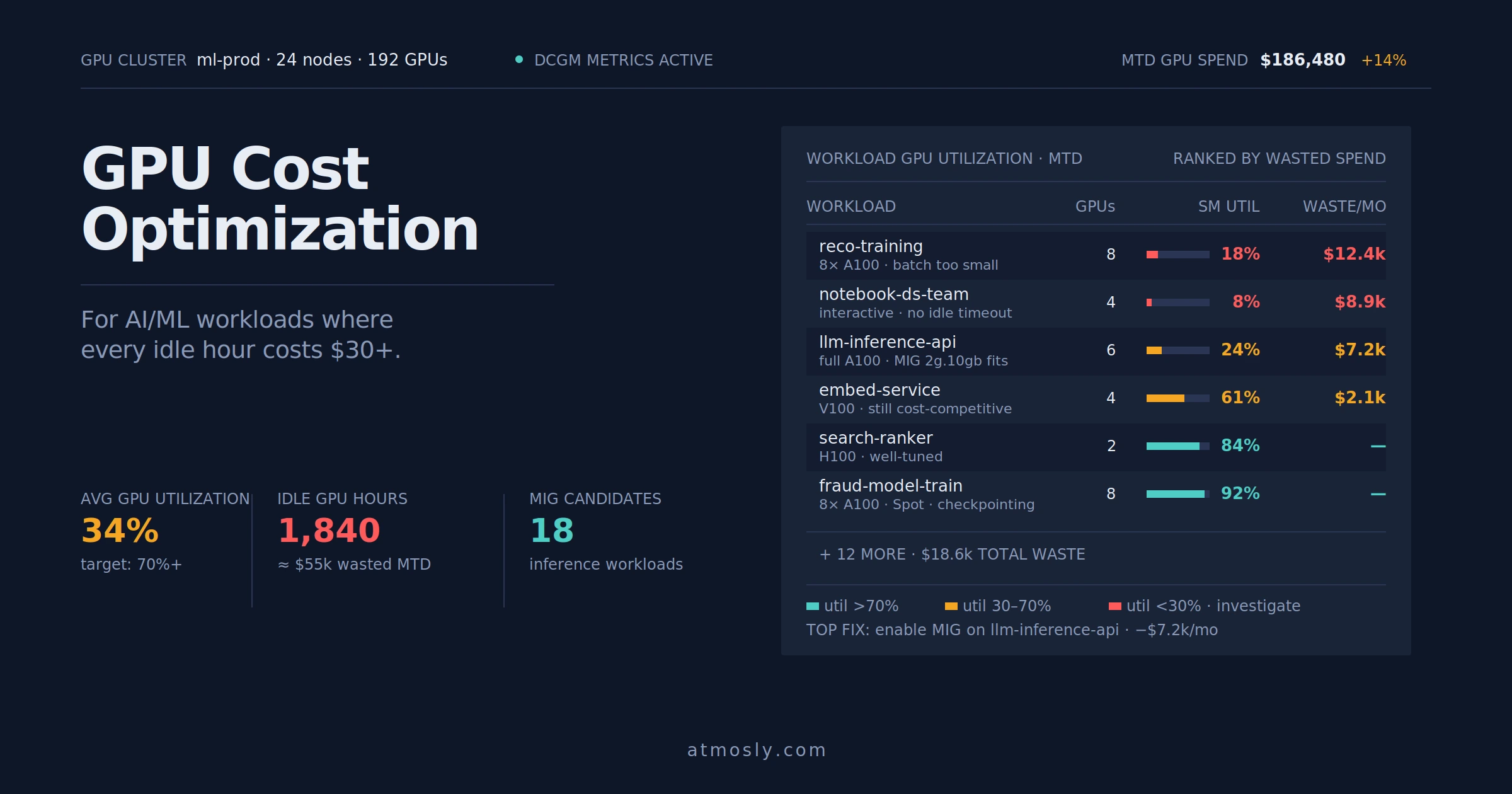
A single A100 node runs roughly $25-30 per hour on major clouds. An H100 node runs $30-40 per hour. A GPU cluster running those nodes 24/7 crosses a million dollars annually before anyone trained a single model that ships to production. Kubernetes GPU cost optimization is the discipline of making sure the money going into those nodes is translating into actual AI/ML output — model training that completes, inference serving real traffic, experiments that produce usable results — rather than idle silicon waiting for jobs that never come, over-provisioned pods holding full GPUs for workloads that need a fraction, and clusters that scale up for peaks and never scale back down.
The economics of GPU workloads are different from CPU workloads in ways that make the standard Kubernetes cost playbook incomplete. A CPU over-provisioned by 3× costs some fraction of a dollar per hour; a GPU over-provisioned by 3× costs $20+ per hour. A CPU workload at 20% utilization is wasteful but survivable; a GPU workload at 20% utilization is the single largest line item on an AI/ML team's budget, and the fix matters by the day, not by the quarter. The surface area is also smaller — fewer workloads, higher per-workload cost — which means fewer places to look but much higher stakes per fix.
This guide covers what actually drives Kubernetes GPU costs for AI/ML workloads, how to detect the specific utilization patterns that signal waste, how to right-size GPU allocations without breaking the training or inference pipelines that depend on them, and the scheduling and autoscaling techniques that keep GPU time productive. The specific mechanics apply whether the GPUs are NVIDIA A100s, H100s, L4s, or the next generation that will have shipped by the time you read this — the economics do not change, even as the hardware does.
The core challenge in GPU cost control is that the signal is weaker than for CPU workloads. CPU utilization is a well-understood number that every monitoring stack reports; GPU utilization comes from NVIDIA's DCGM exporter or equivalent and requires specific setup to flow into the cost pipeline. Teams that want the full picture — GPU time per workload, idle hours by node, model training cost per epoch — without building the pipeline themselves can layer a Kubernetes Cost Optimization platform that handles the DCGM integration, the attribution, and the recommendations. Either way, the mechanics below explain what to look for.
Why Kubernetes GPU Workloads Are Expensive
Several structural reasons make GPU workloads disproportionately expensive compared to CPU workloads, and understanding them is the case for a dedicated optimization program rather than treating GPUs as "just another resource."
The first is the per-hour cost gap. A general-purpose EC2 or GCE instance runs $0.10-0.50 per hour. A single A100 instance runs $25-30 per hour, roughly 100× the rate per node. Every hour that an A100 instance sits idle costs what a general-purpose instance costs in several days of continuous use. The economic consequence of inefficiency is wildly higher for GPU workloads than for CPU workloads, which means the ROI of optimization is also wildly higher per unit of engineering effort.
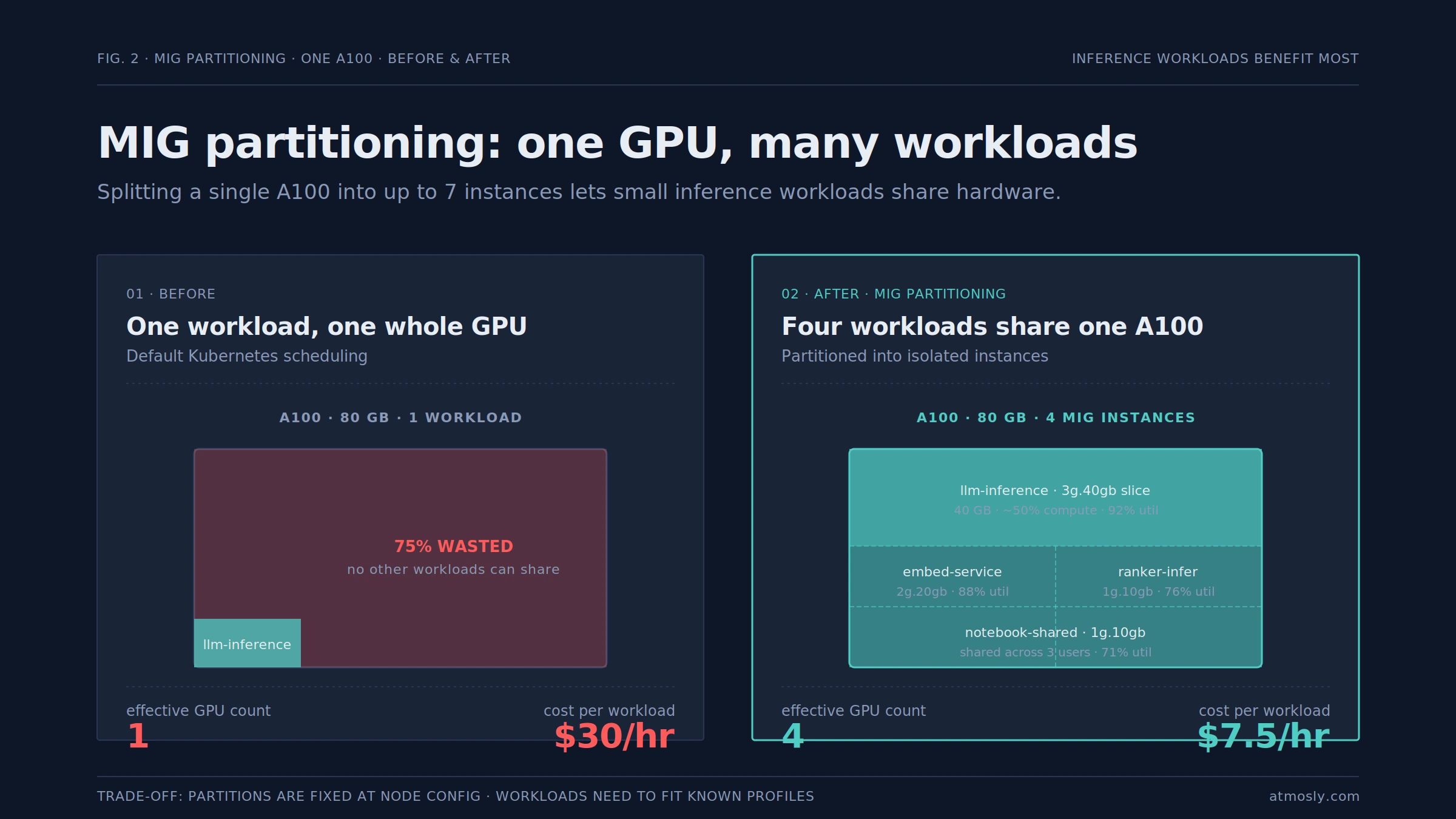
The second is the indivisibility problem. By default, Kubernetes schedules whole GPUs to pods. A workload that needs 20% of a GPU still receives (and bills) 100% of one. In a world of 8-GPU-per-node instances, a single underutilized workload can hold a $30/hour node from being used efficiently. Multi-Instance GPU (MIG) partitioning on A100 and H100 hardware fixes this by letting one physical GPU present as multiple logical GPUs, but it requires explicit setup and only helps if the workloads are small enough to actually fit.
The third is the scheduling gap between training and inference. A training workload wants all the GPUs it can get for a bounded time; an inference workload wants a steady fraction of a GPU for an indefinite time. Running them on the same clusters without separation produces waste — training jobs block inference capacity, inference workloads over-provision for training-peak capacity. Dedicated node pools, taints and tolerations, and separate autoscaling policies for the two patterns are the standard answer.
The fourth is GPU startup time. Spinning up a new GPU node takes 3-5 minutes on major clouds — the instance has to boot, pull the GPU drivers, and warm up CUDA. Workloads that scale aggressively hit this latency repeatedly, which pushes teams toward keeping warm capacity around. Warm capacity that is not actually used is a persistent cost that only shows up in the aggregate monthly bill.
The fifth is the experiment vs. production divide. ML teams run many short exploratory experiments on GPU infrastructure, and the practices that work for training production models (careful rightsizing, long-running jobs, dedicated pools) do not fit experimental work (fast iteration, variable resource needs, interactive sessions). Clusters that only serve one pattern are easier to optimize; clusters that serve both without clear separation accumulate waste from both patterns colliding.
The sixth is the spot interruption cost for GPU workloads. Spot/preemptible GPU instances offer 60-90% discounts, but preemption during a multi-hour training run can cost more in lost progress than the discount saves. Checkpointing frequently enough to make Spot viable adds complexity that CPU workloads do not have. Teams either eat the Spot discount by investing in robust checkpointing, or they pay on-demand prices for the simplicity of guaranteed availability.
How to Identify GPU Underutilization
Finding GPU waste is harder than finding CPU waste because the signal is less visible by default. Three specific sources of utilization data, joined together, tell you what you need.
DCGM metrics are the primary source. NVIDIA's Data Center GPU Manager exports per-GPU utilization, memory utilization, power draw, temperature, and SM (streaming multiprocessor) activity. The DCGM exporter runs as a DaemonSet on every GPU node and ships metrics to Prometheus. Without DCGM in the pipeline, GPU utilization is effectively invisible — the Kubernetes resource accounting shows that a pod has one GPU allocated but says nothing about whether that GPU is doing anything.
Pod-level resource attribution is the second source. Which pod is using which GPU, for how long, with what workload type (training, inference, experiment). This comes from standard Kubernetes labels joined with DCGM's per-GPU attribution. The join is critical — DCGM reports utilization per GPU, Kubernetes reports pod-to-node mapping, and the pipeline needs both to say "the recommender-training workload used 80% of GPU 3 on node A for 4 hours."
Node-level scheduling data is the third source. How much time nodes spend running GPU workloads versus sitting idle waiting for jobs. A node that is up for 24 hours but only runs GPU workloads for 10 of them is 58% wasted at the node level, before any workload-level utilization matters. Cluster Autoscaler and Karpenter logs show the scaling behavior; node-level allocation metrics show whether the scaling matched demand.
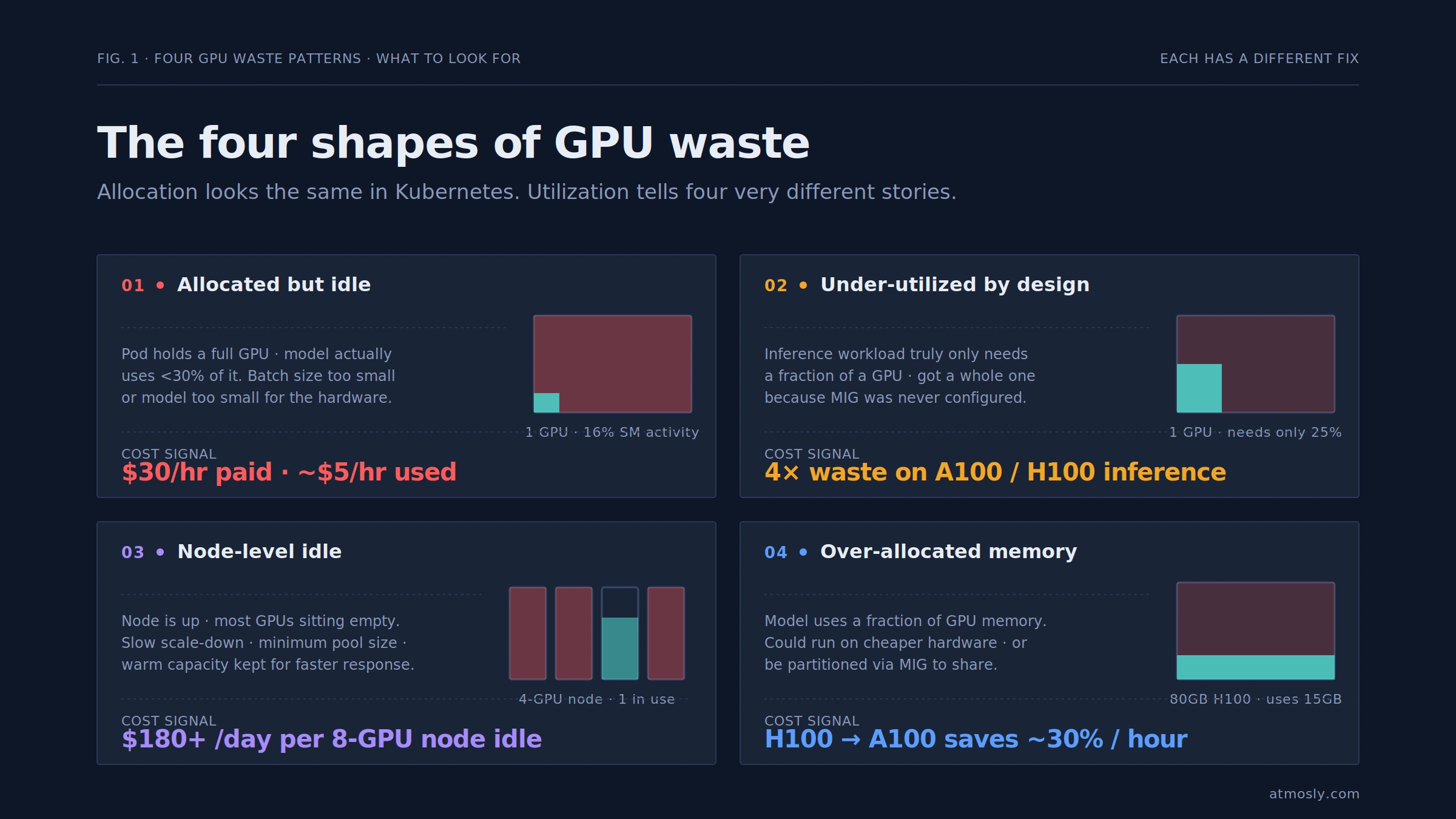
With these three sources, the specific patterns of GPU waste become visible. Allocated-but-idle is the most expensive and most common: a pod is holding a GPU but running something that uses less than 30% of it, often because the batch size was set conservatively or the model is too small for the hardware. Under-utilized by design: inference workloads that genuinely need less than a full GPU but get a whole one because MIG was never set up. Node-level idle: GPU nodes staying up for policy reasons (minimum node pool size, slow scale-down configurations) when there are no workloads to run. Over-allocated memory: GPU memory requests set far above actual usage, which looks like efficient utilization in some dashboards but still blocks other workloads from sharing the GPU.
For CPU-side waste, the same investigative discipline applies in parallel — many of the specific kubectl and jq techniques for finding orphaned resources and idle capacity transfer directly to GPU-adjacent CPU workloads, and are covered in the Kubernetes idle resources playbook.
Right-Sizing GPU Resources for AI/ML Workloads
Once you know which workloads are under-utilizing their GPUs, the rightsizing work is specific to the workload pattern. The approach for training differs from the approach for inference differs from the approach for experimentation.
Training workloads benefit most from batch size tuning and framework-level optimization before considering rightsizing. A training job that uses 20% of a GPU often has room to double or triple the batch size, which uses more GPU utilization per hour and completes the training faster at the same hourly cost. Framework-level techniques like mixed precision training (FP16/BF16 instead of FP32), gradient accumulation, and data loading parallelism increase effective GPU utilization without changing the hardware allocation. Only after these techniques are exhausted does the hardware rightsizing conversation make sense — moving a workload from an A100 to an L4, or from H100 to A100.
Inference workloads are the natural fit for MIG partitioning. A single A100 can be partitioned into up to 7 instances (1g.5gb, 2g.10gb, 3g.20gb, etc.), each presenting as a separate GPU to Kubernetes. An inference workload that only needs 10GB of GPU memory and modest compute can run on a 2g.10gb slice instead of a full A100, letting the other 60GB serve other workloads. The configuration is set at the node level and workloads request specific MIG profiles via resource specs. Teams running significant inference workloads on A100/H100 without MIG are typically paying 3-5× what they need to.
Experimentation and interactive workloads are hardest to rightsize because the usage pattern is intentionally variable — the whole point of experiments is to try different approaches. The pattern that works is dedicated node pools for interactive work with aggressive scale-to-zero policies when sessions end, plus GPU time-slicing (available on non-MIG hardware or on top of MIG) that lets multiple notebooks share a GPU. Interactive sessions that run on dedicated-GPU allocations with 10% utilization are the single largest category of waste in most ML team's budgets.
Memory sizing matters as much as compute sizing. GPU memory is the hard constraint — a model that needs 60GB of GPU memory will not fit on a 40GB A100 regardless of how much compute it uses. The rightsizing check is whether the workload's actual memory usage justifies the hardware choice. A workload using 15GB on an 80GB H100 is paying for 65GB of unused memory for the entire training run. Model quantization, gradient checkpointing, and ZeRO offloading can reduce memory requirements and let workloads fit on cheaper hardware.
Hardware generation choice is a per-workload decision. Not every workload needs H100 performance. L4s and T4s are much cheaper per hour and handle most inference workloads well. V100s remain cost-competitive for many training workloads that do not need A100/H100 specific features. The rightsizing question is not "what is the best GPU" but "what is the cheapest GPU that meets the workload's actual requirements."
Using Scheduling and Autoscaling to Reduce GPU Costs
Once individual workloads are rightsized, scheduling and autoscaling decisions determine how efficiently the fleet of GPUs is used in aggregate. Several specific techniques reliably reduce GPU costs without reducing throughput.
Dedicated GPU node pools with taints. GPU nodes should be tainted so that only workloads explicitly tolerating the taint can land on them. This prevents CPU-only workloads from accidentally scheduling on expensive GPU nodes and taking up capacity that should serve GPU workloads. The pattern is standard: a nvidia.com/gpu=true:NoSchedule taint on GPU nodes, matching toleration on pods that need GPUs.
Separate pools for training vs. inference vs. interactive. Training wants large bursts of capacity for bounded time; inference wants steady capacity indefinitely; interactive wants small bursts of capacity with aggressive scale-down. These three patterns do not share pools well. Separate node pools with pattern-specific autoscaling policies — fast scale-up and scale-down for interactive, longer scale-down windows for inference, batch-oriented provisioning for training — let each pattern use the fleet efficiently.
Priority classes and preemption. Running experiments on a cluster with production inference workloads needs a priority model. Production inference gets a high priority class with guaranteed capacity; batch training gets medium priority and runs on capacity that production is not using; interactive experiments get low priority and are preempted when higher-priority work needs the capacity. This is standard Kubernetes priority class setup, with the twist that preemption on GPU workloads needs to interact with checkpointing to avoid losing significant progress.
Scale-to-zero for infrequent inference endpoints. Inference services with sporadic traffic are expensive to run at always-on minimum replicas. KServe, Seldon, or similar serving platforms support scale-to-zero with a cold-start penalty when traffic arrives. For endpoints that see traffic in bursts and are idle for hours between, scale-to-zero can cut cost by 80%+. The cold-start latency (loading model weights into GPU memory on the first request) is the trade-off; for internal tools and non-latency-critical endpoints, this is usually acceptable.
Spot/preemptible nodes with robust checkpointing. GPU Spot instances offer 60-90% discounts. For workloads that can checkpoint and resume, this is the single largest cost reduction available. The checkpointing has to be frequent enough that preemption loses only a few minutes of work, which usually means checkpointing every 100-500 training steps depending on the model size. The engineering investment pays back quickly for workloads with sufficient volume.
Cluster autoscaler tuning for GPU nodes. The default Cluster Autoscaler and Karpenter configurations are tuned for CPU workloads where scale-up takes seconds. GPU nodes take 3-5 minutes to come up with drivers loaded. Scale-up for GPU workloads needs to be proactive — provisioning capacity before the queue builds up — and scale-down needs to be more conservative to avoid thrashing on short gaps between jobs. Tuning the autoscaler for GPU-specific latencies prevents both over-provisioning (keeping too much warm capacity) and under-provisioning (jobs waiting for nodes to spin up).
Job queueing with Kueue or Volcano. Batch training workloads benefit from a queue system that orders and schedules jobs across available capacity rather than requesting resources immediately. Kueue (standard Kubernetes job queueing) and Volcano (batch-oriented scheduling) both let teams submit many training jobs and have them packed efficiently onto available GPUs, maximizing utilization during busy periods and minimizing idle time between jobs.
The specific pattern of catching cost anomalies in real time applies to GPU workloads too — a training job that was supposed to finish in 6 hours and is still running at hour 20 represents significant unexpected cost. The same rolling-baseline anomaly detection that catches runaway CPU costs catches runaway GPU costs, with the added signal of DCGM utilization patterns to distinguish "running efficiently but longer than expected" from "stuck in a loop burning GPU for no output."
Best Practices for Kubernetes GPU Cost Optimization
The teams that keep GPU costs under control over time share a few habits that teams struggling with it usually do not.
They measure utilization at the GPU level, not just the pod level. A pod allocated one GPU looks like 100% utilization in Kubernetes resource accounting — the resource is fully allocated. Measuring DCGM-reported SM activity, memory utilization, and power draw is what reveals whether the GPU is actually doing work. Teams that only track Kubernetes-level allocation miss the entire category of allocated-but-idle waste, which is usually the largest.
They separate experiment and production clusters when the scale justifies it. Experimentation produces chaotic utilization patterns; production serving produces predictable patterns. Running both on the same cluster means neither pattern can be optimized well. For teams at sufficient scale, splitting into dedicated clusters per pattern reduces interference and makes each cluster easier to optimize.
They set hard quotas on experimental GPU time. A data scientist running a notebook that holds a full A100 for a week without actually using it is one of the most common patterns of GPU waste. Namespace-level ResourceQuotas, time-limits on interactive sessions enforced by cluster-level policy, and automatic cleanup of idle notebooks prevent the pattern from running indefinitely.
They right-size continuously, not just at launch. Model architectures change, batch sizes evolve, inference traffic patterns shift. A rightsizing decision that was correct six months ago may be wrong today. Rightsizing recommendations should regenerate against the latest utilization data monthly and ship as PRs the owning team can review, not as a one-time project.
They make GPU cost visible per model, not just per cluster. A fleet-level view that shows total GPU spend tells the platform team how much they spent; a per-model breakdown tells the ML team which models are expensive to serve. This translates directly into business decisions — a model that costs $8k/month to serve may be worth it or may not depending on the business value it produces, but someone has to be able to see the number.
They integrate cost into model evaluation. The teams that treat GPU cost as a model-performance metric alongside accuracy and latency produce more efficient models. A model that is 1% more accurate but 3× more expensive to serve is often the wrong choice; a slightly less accurate model with better inference economics is often right. This decision happens at model selection time and needs cost data available in the ML evaluation pipeline.
They plan for hardware generation shifts. GPU hardware changes faster than most infrastructure. H100 was released in 2022 and became mainstream in 2024; the next generation is already being deployed. Teams that lock into specific hardware without a migration plan end up paying premium prices for aging hardware when newer, cheaper options exist. Annual review of hardware allocation against the current cloud catalog surfaces opportunities to migrate workloads to cheaper equivalents.
NVIDIA's documentation on MIG and GPU partitioning covers the specific mechanics of GPU slicing that most inference workloads benefit from. The configuration is well-documented but requires explicit setup — it is not on by default.
See what your GPU hours are actually doing.
Connect a GPU cluster read-only and get per-workload GPU utilization, allocated-but-idle hours, MIG recommendations, and ranked rightsizing candidates by dollar impact. Setup takes a few minutes. Try it free →