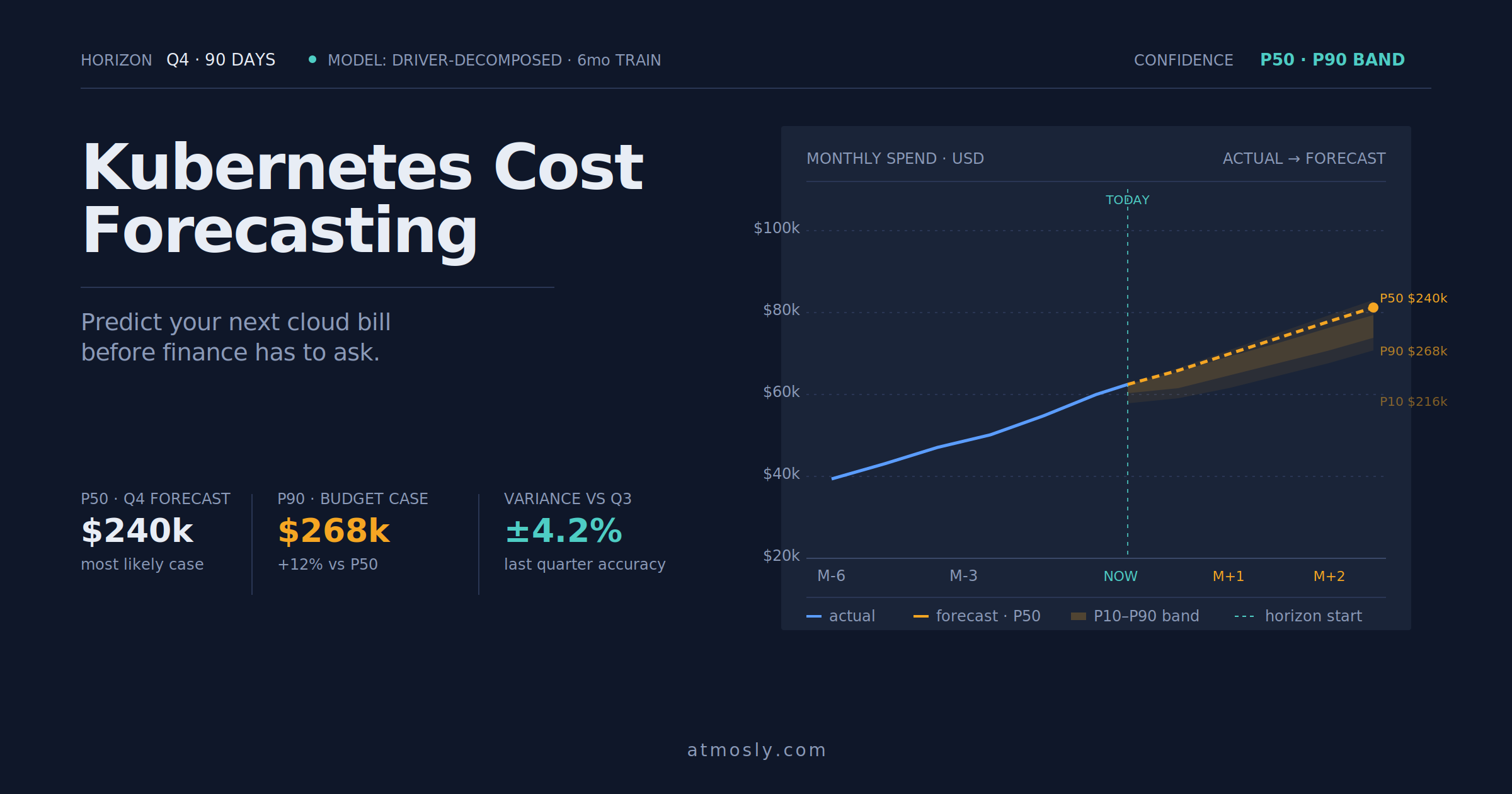
Every quarter, someone in finance asks the platform team what Kubernetes will cost next quarter, and the answer is usually a range wide enough to be useless. "Somewhere between $180k and $260k, depending on traffic" is not a number anyone can budget against. Kubernetes cost forecasting is the discipline of narrowing that range — not to a single point, which would be false precision, but to a defensible band with the assumptions written down and the drivers named, so that when the actual bill lands, the variance is small enough to explain and the surprises are the ones that were flagged upfront.
The reason this is harder in Kubernetes than in traditional infrastructure is that the bill is downstream of decisions no single team owns. Traffic drives HPA replicas, which drive node count, which drives compute cost. New deployments carry copy-pasted resource requests that inflate the cluster's memory reservation whether the workload uses it or not. A CI pipeline that started creating ephemeral namespaces last week is already priced into next month's bill, but nobody has told the person doing the forecast. Cost prediction on top of this substrate needs to model the drivers, not just extrapolate the totals.
This guide covers what "forecasting" actually means for a Kubernetes environment, what data you need to build one that is useful rather than decorative, and the specific error modes that make most first attempts embarrassing. Most of the mechanics translate across cloud providers; the model quality translates across tools. What does not translate is the discipline of writing the assumptions down and reviewing the variance every month.
The single largest lever in accurate forecasting is the quality of the underlying attribution — you cannot forecast at the workload level if you cannot allocate at the workload level today. Teams that want the forecast maintained continuously instead of rebuilt every quarter can layer a Kubernetes Cost Optimization platform on top of the cluster, and get the projection, the confidence bands, and the variance report as an output of the same pipeline that drives rightsizing and anomaly detection. Either way, the mechanics below are what actually produce a defensible number.
What Is Kubernetes Cost Forecasting?
Kubernetes cost forecasting is the practice of estimating future cluster spend across a defined horizon — usually the next month, quarter, or fiscal year — using historical usage, known upcoming changes, and models of how the workload will grow. The output is not a single number. It is a projection with a confidence interval, decomposed by cost category (compute, storage, network, management fees) and attributed to the drivers most likely to move it.
There are two distinct use cases, and mixing them up is where most forecasting programs go wrong. Budget forecasts are the number finance uses to plan cash flow and set spend caps. They need to be conservative — closer to the P90 than the median — because underestimating the budget produces a mid-quarter overrun conversation, while overestimating just leaves headroom. Operational forecasts are the number the platform team uses to decide when to buy Committed Use Discounts, when to expand capacity, or when a cost trajectory needs intervention. They need to be closer to the P50 with wider confidence bands, because the goal is to make the best decision on average, not to protect against every tail scenario.
A forecast is only as good as the assumptions behind it. A number that says "next quarter will be $240k" tells you nothing about what would falsify it. A useful forecast says "next quarter is $240k plus or minus $28k, assuming P50 traffic growth of 8% month-over-month, no major new services launching, and the Spot VM migration currently in progress lands by month two." When the actual bill comes in outside that range, you know exactly which assumption broke, and the next forecast gets more accurate. Without written assumptions, the forecast is just a guess with more decimals.
What Data Is Needed to Forecast Kubernetes Costs?
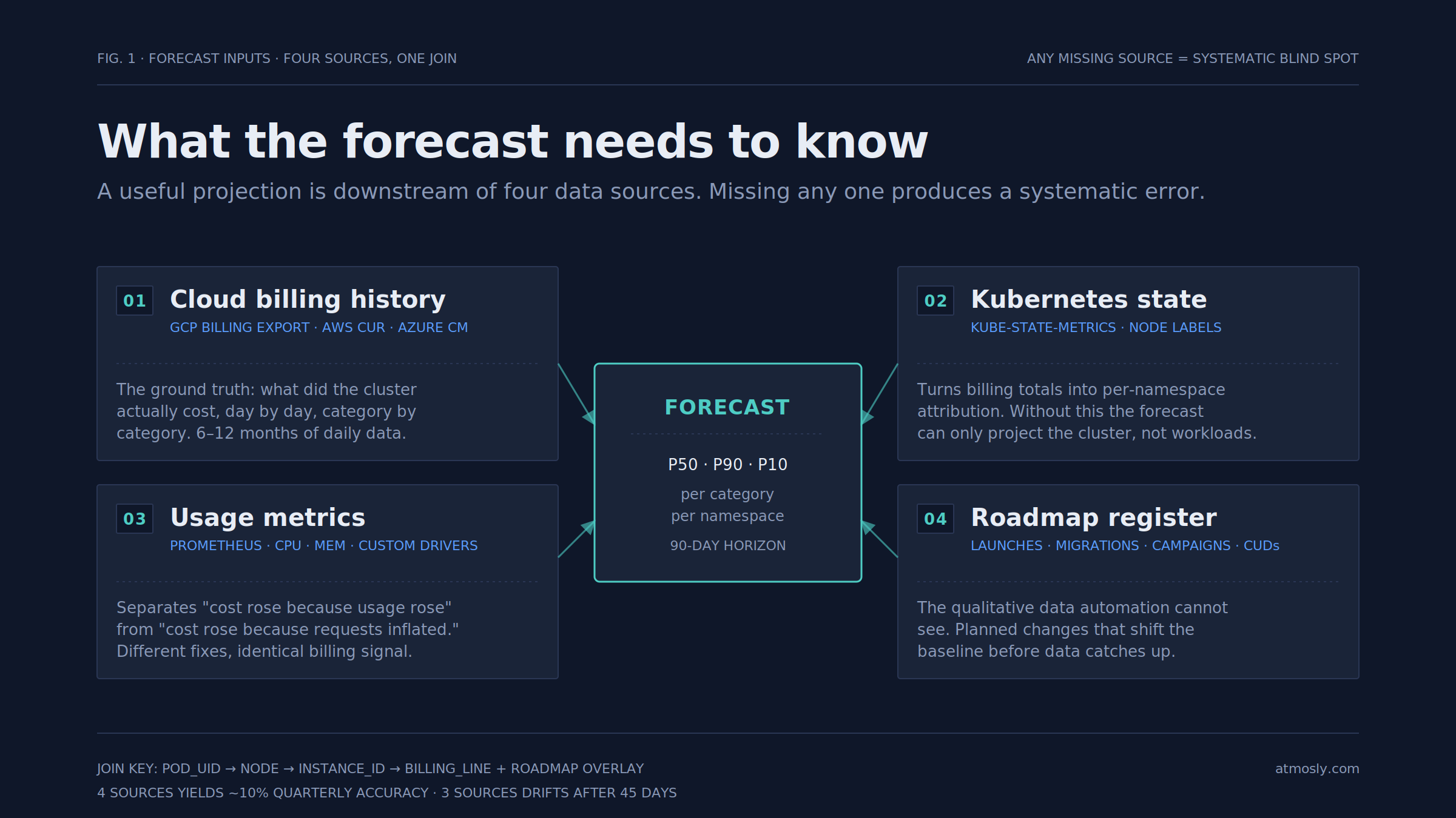
A good forecast needs four data sources joined together, and the join is usually the hard part. Cloud billing tells you what was spent; Kubernetes state tells you what ran; usage metrics tell you how hard the workloads worked; and roadmap inputs tell you what will change. Any forecast built on three of these instead of four will systematically miss the fourth's failure mode.
Cloud billing history is the starting point. Google Cloud Billing Export, AWS Cost and Usage Report, or Azure Cost Management data — daily or hourly, exported to a data warehouse — gives you the ground truth of what the environment cost. Twelve months of history is enough to model seasonality; six months is workable for younger workloads; less than three months means the forecast will be dominated by whatever happened in the last few weeks, which is usually not representative.
Kubernetes state history is what turns billing totals into per-workload attribution. kube-state-metrics snapshots joined with node labels and pod-to-namespace mappings let you say "this $80k of last month's compute was the payments-api namespace, this $60k was analytics." Without this, the forecast can only say "the cluster will cost more next quarter" — useful directionally, useless for the team that needs to decide whether to launch a new service.
Usage metrics come from Prometheus or the equivalent. CPU and memory usage per workload, request rate, queue depth, and any custom business metrics that drive scaling behavior. The forecast uses these to distinguish two very different situations that look identical on the billing side: cost went up because usage went up (expected; forecast should follow the trend), and cost went up because requests were inflated but usage stayed flat (waste; forecast should reflect the fix that is coming).
Roadmap inputs are the qualitative data that automated systems cannot see. A new service launching next month, a migration off a legacy database, a marketing campaign expected to drive 3× traffic for two weeks, a Spot VM migration currently in progress. Every serious forecast has a "known changes" register that names each planned event, its expected cost impact, and its confidence level. Forecasts that ignore roadmap data drift out of accuracy within one quarter because the world stops matching the training data.
The mechanics of joining billing to Kubernetes state are the same ones that drive per-namespace cost allocation, and the showback and chargeback playbook covers that pipeline in detail. If the attribution is not working for allocation, it will not work for forecasting either — they are the same problem.
How to Predict Future Kubernetes Cloud Spend
The mechanics of the forecast itself range from a spreadsheet to a machine learning model, and the honest answer is that the spreadsheet is usually good enough. Most teams overreach for sophistication when the accuracy problem is upstream in the data quality.
The baseline projection is the simplest useful forecast. Take the last three to six months of daily spend, fit a linear or exponential trend, and project it forward across the horizon. This works because most Kubernetes workloads grow relatively smoothly outside of specific events, and a well-fit trend captures 70-80% of the signal for the coming quarter. Where it breaks is when the recent history has a bend that the trend cannot see — a rightsizing project that just finished, a service that just migrated to Spot, a namespace that just doubled its replicas.
Component decomposition improves accuracy by forecasting each cost category separately and summing. Compute usually grows roughly with workload volume, storage grows more slowly and monotonically, network egress can spike based on architectural changes, and management fees are flat unless cluster count changes. A forecast that sums independent per-category projections is meaningfully more accurate than a single-line total forecast, because each category's trend is closer to linear than the aggregate is.
Driver-based modeling is the next step up. Instead of forecasting cost directly, forecast the drivers — traffic, active user count, transaction volume, whatever the business tracks — and translate them into cost via a per-driver unit-cost multiplier. This is the forecasting method that actually explains variance when the number comes in different from expected, because you can trace back to which driver moved. If active users came in 20% higher than expected and cost came in 15% higher, the model is working; if active users were flat and cost was up 20%, something else is going on and the forecast alerted you to look.
Scenario forecasts wrap the base projection with explicit alternates. A P50 case (most likely), a P90 case (higher spend if growth accelerates or a planned optimization slips), and a P10 case (lower spend if a planned migration lands early or a service is deprecated). Finance uses the P90 for budgeting; the platform team tracks against P50; both refer to the same underlying model. This structure also forces the assumptions to be written down, because moving between scenarios requires naming what would change.
Confidence bands are the piece most teams skip and most later regret. A single-point forecast has no way to communicate uncertainty; the audience defaults to treating it as precise, and every deviation feels like a failure. A band — even a rough one, like ±15% for the current quarter and ±30% for two quarters out — sets the right expectation and turns the conversation from "the forecast was wrong" to "we ended up at the upper edge of the band, here is why."
None of this needs machine learning. Most teams get to 90% of the useful accuracy with time-series decomposition and per-driver modeling in a spreadsheet or a scheduled BigQuery job. Reach for ARIMA or Prophet when you have a clear seasonal pattern that simpler methods do not capture, and remember that a more complex model with the same data quality will not fix the data quality problem.
Factors That Can Cause Cost Forecasting Errors
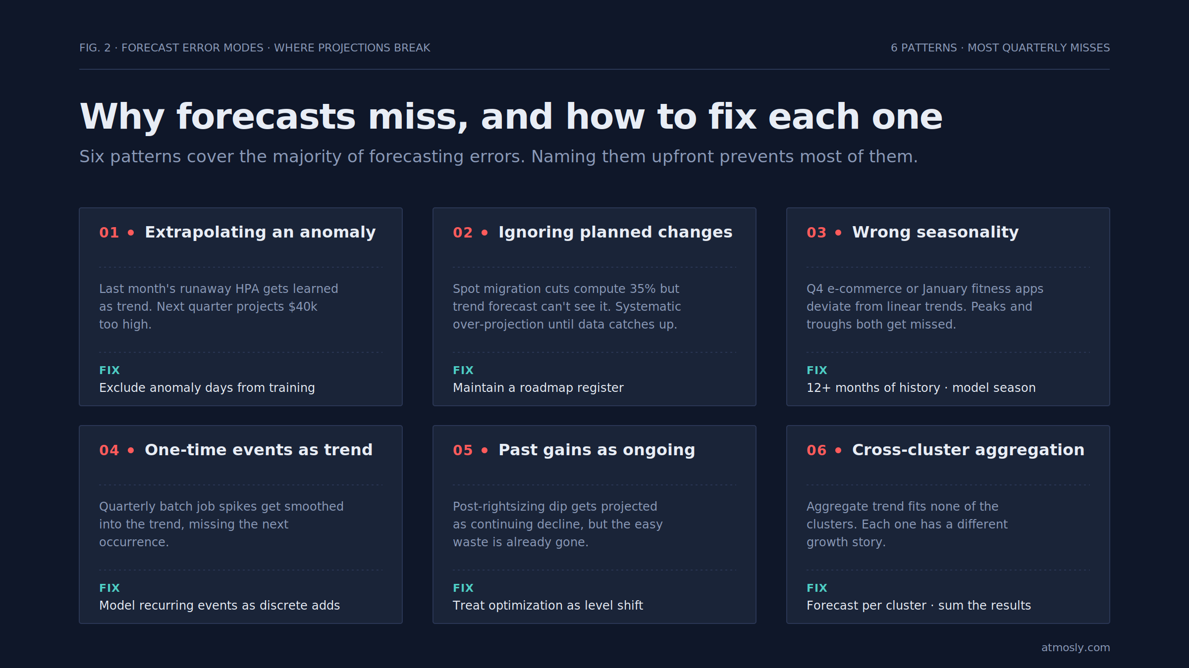
Forecasts miss for a small number of repetitive reasons, and knowing them in advance is most of the defense against them. Six patterns produce the majority of forecasting errors worth caring about.
Extrapolating a recent anomaly is the most common mistake and the easiest to make. Last month's bill included a runaway HPA that ran for four days before being caught. If the forecast includes that spike in the training window, it will project the anomaly forward, and next quarter's forecast will be $40k too high. Anomaly detection running upstream of the forecast — the same kind of real-time anomaly detection that catches runaway spend day-of — should also flag those days for exclusion from the forecast training data.
Ignoring planned changes produces the opposite error. The Spot VM migration currently in progress will cut compute by 35% once complete, but a pure trend forecast has no way to see it. The forecast trend continues at pre-migration cost, the actual bill drops, and the forecast systematically over-projects until enough post-migration data lands to update the trend. This is why the roadmap register matters — a forecast that adjusts the trend by the expected impact of a known change is more accurate than one that waits for the data.
Wrong seasonality assumptions hurt forecasts for consumer-facing workloads especially. Traffic patterns in Q4 for e-commerce, in January for fitness apps, and in September for education platforms deviate meaningfully from the rest of the year, and a forecast that treats every month as equivalent will miss the peaks and the troughs. At least twelve months of history is what makes yearly seasonality visible; less than that means the forecast should not claim to model it.
One-time events treated as trend. A quarterly batch job that runs for three days at 10× normal load will appear in the training data as a temporary spike. A naïve trend will either project the spike forward (over-forecasting) or smooth it away (missing the next occurrence). Marking recurring events explicitly and forecasting them as discrete additions to the baseline is more accurate than trying to make the trend absorb them.
Rightsizing gains that already peaked. Teams that recently completed a rightsizing sprint see their bill drop and their forecast get more optimistic. Then the forecast keeps assuming further optimization gains that are not coming, because the easy waste is already gone. Forecasts should treat past optimization as a level shift, not an ongoing trend, unless there is a specific reason to expect it to continue.
Cross-cluster or cross-project mixing. A forecast built on aggregated spend across three clusters that grew at different rates will fit a trend that matches none of them. Forecasting each cluster or each project separately and summing produces better accuracy meaningfully, especially when the clusters have different workload profiles or growth rates.
Best Practices for Accurate Kubernetes Cost Forecasting
The teams that produce forecasts finance can actually plan against share a small number of habits, and the ones that produce forecasts that get quietly ignored share the opposite ones.
They rebuild the forecast on a fixed cadence rather than treating it as a set-and-forget artifact. Monthly is the minimum for a forecast that stays useful; weekly is better for fast-growing environments. Each rebuild incorporates the latest actuals, updates the roadmap register, and produces a variance report against the previous forecast. The variance report is often more valuable than the forecast itself, because it is where you learn which assumptions to trust.
They decompose accuracy by category. A forecast that is 3% off in total might be 10% too high on compute and 7% too low on egress, netting to 3% by accident. Tracking accuracy per category surfaces the model's real strengths and weaknesses and points at which part of the pipeline needs the next round of investment.
They make the assumptions explicit and separable. The best forecast documents are the ones where you can point at a specific line item, see what assumption drives it, and change that assumption to see the number update. A forecast that reads as a black box gets treated as one, and nobody defends it when the number comes in wrong.
They integrate the forecast with anomaly detection so that both use the same baseline. A forecast that says the next quarter will be $240k and an anomaly detector that says today's spend is 40% above baseline should be talking about the same baseline; otherwise, the two systems disagree about what "normal" looks like and the team loses trust in both.
They treat optimization as a forecast input, not a separate track. A rightsizing project that will land in month two of the quarter reduces the forecast for months two and three, with a stated confidence level on the landing date. Optimization work that is not reflected in the forecast is optimization work that finance is not counting on — and if it lands late, no one is surprised, but if it lands on time, the platform team gets no credit because nobody was expecting the improvement.
They feed the forecast back into commitment decisions. Committed Use Discounts on GCP and Reserved Instances or Savings Plans on AWS need a defensible baseline forecast to size correctly. Over-committing wastes the discount because you pay for capacity you do not use; under-committing leaves savings on the table. The forecast is the input that turns commitment sizing from a guess into a decision.
Google Cloud's guidance on FinOps and cost management covers the broader budgeting and cost-control practices that a forecast plugs into. The forecast is one input to that program, not the whole program.
Get a forecast you can actually defend.
Connect a cluster read-only and get a 90-day forecast, decomposed by namespace and cost category, with confidence bands and a variance report against your last forecast. Setup takes a few minutes; no cluster changes. Try it free →